Power Law: The Hidden Rule Behind Extreme Outcomes

What Is a Power Law? The Simple Explanation

Have you ever noticed that a few cities hold most of a country’s population? Or that a handful of blockbuster movies earn most of the box office revenue? Or that a tiny number of people own a huge share of the world’s wealth? These patterns all follow a power law.

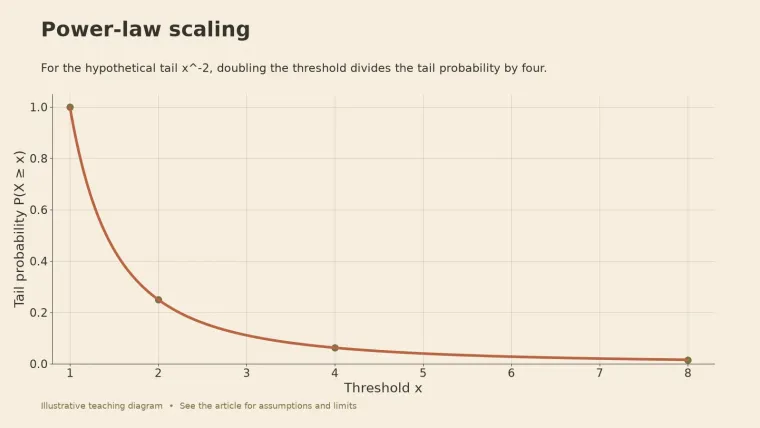
In simple terms, a power law is a relationship between two quantities where a relative change in one leads to a proportional relative change in the other, no matter how big or small the starting numbers are. It’s a pattern where small things are extremely common, and large things are extremely rare—but the large things are so large that they dominate the total.

Think of it this way: if you lined up all the cities in the US by population, you’d see a few giants like New York and LA, then a long tail of smaller cities. The biggest city isn’t just a little bigger than the next one; it’s many times bigger. And that gap keeps shrinking as you go down the list, but the pattern stays the same.

That’s the essence of a power law: the rich get richer, and the big get bigger — not by a fixed amount, but by a fixed proportion.

The Math Behind the Magic

Mathematically, a power law is written as:

y = a × x^k

Where:

• y is the result (like city population or wealth)
• x is the variable (like rank or size)
• a is a constant
• k is the exponent (often called alpha, α)

The exponent is the key. It determines how unequal the distribution is. A smaller exponent (like 1 or 1.5) means a fatter tail—more extreme outliers. A larger exponent (like 3 or 4) means a thinner tail—less extreme differences.

Earthquakes are the cleanest example, and they are worth getting right. The Gutenberg-Richter law says that for every magnitude 6 quake there are roughly ten magnitude 5s, a hundred magnitude 4s, and so on: the count falls about tenfold per magnitude step, which is the exponent (seismologists call it the b-value) sitting close to 1 in most regions. The energy runs the other way. According to the US Geological Survey, each whole step up the magnitude scale releases about 32 times more energy, not 10 times.

So one step up makes an event ten times rarer and roughly thirty times more violent. That mismatch — rarity falling slower than severity rises — is why a handful of quakes cause most of the damage, and it is the same mismatch behind every other example in this article.

Another classic example is word frequency in a language. The most common word (‘the’) appears about twice as often as the second most common (‘of’), and three times as often as the third, and so on. This is known as Zipf’s law, a special case of a power law.

Why Power Laws Matter: The ‘Big Deal’ Explained

Power laws get attention because they break an intuition almost everyone carries around. We are trained to think in bell curves — the normal distribution — where most values cluster near an average and extremes are both rare and mild.

But power laws describe a world where extremes are not just possible; they’re expected. In a power law world there is no “average” that represents the typical case. A few huge values pull the mean somewhere that describes nobody.

Consider wealth. Height behaves itself: line up 100 people and nobody is 10 metres tall, so the group’s average height genuinely describes the group. Wealth does not behave itself. Add one billionaire to the same 100 people and the average net worth in the room jumps by millions, while the typical person is exactly where they were.

This is measurable, not rhetorical. When researchers fitted the Forbes 400 list, the wealth of the richest Americans followed a Pareto (power-law) distribution with an exponent of about 1.49 (Klass and colleagues, Economics Letters, 2006) — low enough that the average is carried almost entirely by the top of the list.

This has huge implications for how we understand risk, success, and even natural disasters. It means that the biggest events—like a pandemic, a market crash, or a blockbuster hit—are not anomalies but part of the same pattern that produces small events.

Real-World Examples of Power Laws

Power laws appear everywhere once you start looking:

• City sizes: City populations follow Zipf’s law, and for US metropolitan areas the exponent has stayed close to 1 for about a century (Gabaix, Quarterly Journal of Economics, 1999). The fit is strongest among the largest cities; further down the list a lognormal often describes the data better, and a 2020 study found the US exponent has been drifting as smaller cities grow (Hackmann, Papers in Regional Science, 2020).
• Wealth distribution: The top of the wealth distribution is the classic power-law tail — it is why the top 1% holds a share out of all proportion to its size. The Federal Reserve’s Distributional Financial Accounts publish that share every quarter.
• Earthquake magnitudes: The Gutenberg-Richter law, with roughly ten times fewer events per magnitude step.
• Word frequencies: In any language, a small set of words does most of the work. This is Zipf’s law, and it is one of the better-behaved examples when tested properly.
• Website traffic: A few sites take most of the traffic while millions get almost none.
• Book sales: Circana BookScan data reported by The New York Times in 2021 showed that 98% of the titles publishers released in 2020 sold fewer than 5,000 copies; Bookstat figures widely quoted in 2024 put roughly 96% of books under 1,000 copies.
• Social media followers: A few accounts have millions of followers; most have a handful.
• Bitcoin price: Some analysts fit Bitcoin’s price to a power law of time. That claim is contested, and the FAQ below explains why the evidence is weaker than the chart looks.

Power Law vs. Normal Distribution: Spot the Difference

It’s easy to confuse power laws with normal distributions, but they’re fundamentally different.

In a normal distribution, most values cluster around the mean, and the probability of extreme values drops off exponentially. For example, human heights follow a normal distribution: most people are around 5’5” to 5’10”, and very few are 7 feet tall.

In a power law, there is no typical value. The distribution is ‘heavy-tailed,’ meaning that extreme values are much more likely than in a normal distribution. For example, the number of citations a paper receives follows a power law: most papers get few citations, but a tiny number get thousands.

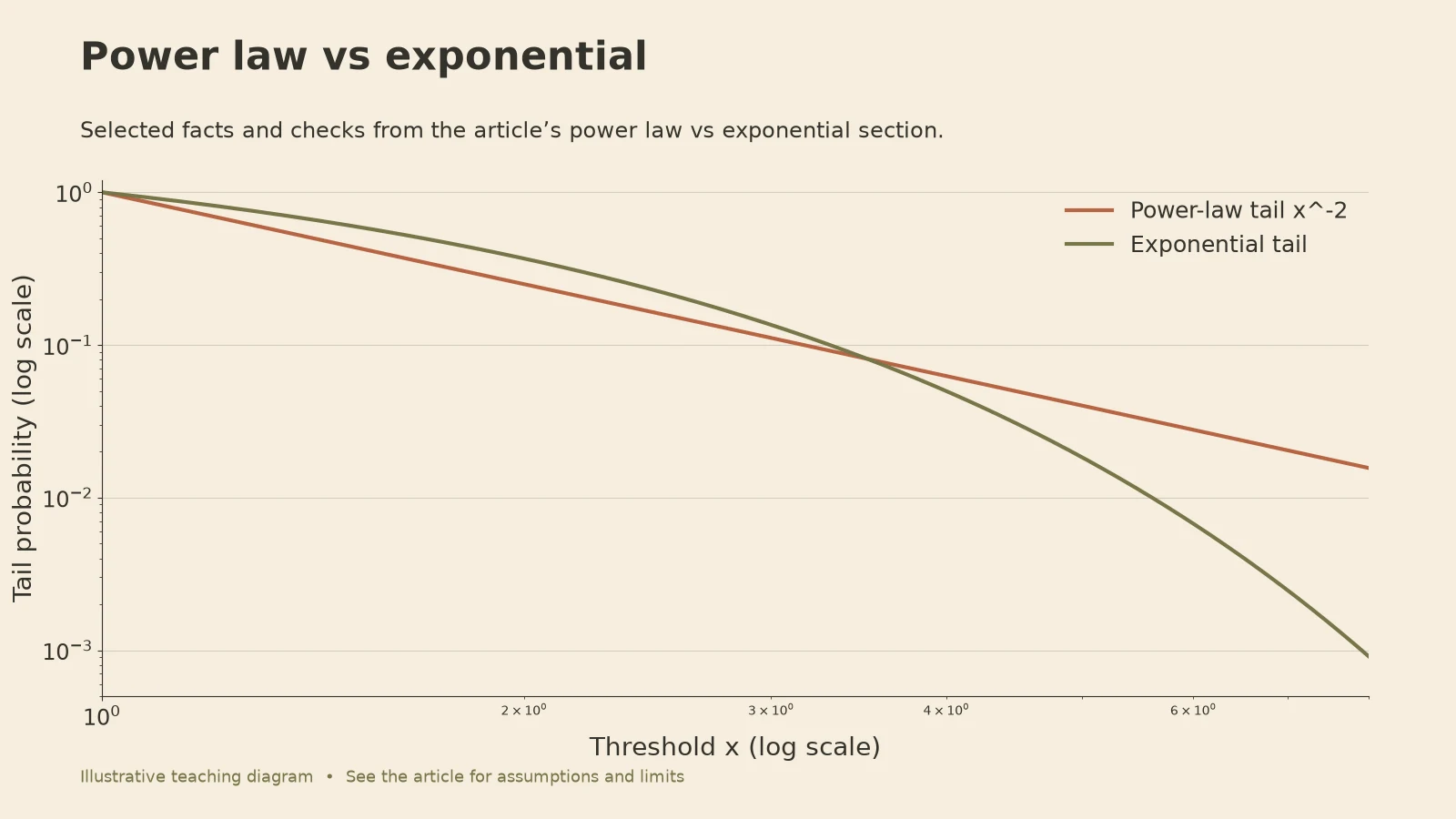
One way to tell them apart is to plot the data on a log-log graph, where each step along an axis means multiplying rather than adding. A power law straightens out into a line. A normal distribution bends away sharply.

One warning before you use that trick: a straight-ish line on a log-log plot is where the investigation begins, not where it ends. This is the single most common way people get power laws wrong, so it deserves its own section.

Before You Call It a Power Law: Most Claims Fail the Test

This is the part that rarely makes it into explainers, and it is the part that will save you from a bad decision.

In 2009, Aaron Clauset, Cosma Shalizi and Mark Newman took 24 datasets that were widely cited as power laws — from physics, biology, earth science, computing and the social sciences — and tested them properly (SIAM Review 51(4), 661–703). Some were consistent with a power law. Several were ruled out. Several more were borderline: a power law was possible, but the data did not support it strongly. Eyeballing a log-log plot could not tell these cases apart, which is exactly why so many of the original claims had stuck.

The same authors later widened the net. Broido and Clauset examined nearly a thousand network datasets and concluded that genuinely scale-free structure is rare, with alternative distributions fitting at least as well in most cases (Nature Communications 10:1017, 2019).

The rival you have to rule out is the lognormal

A lognormal distribution comes out of ordinary multiplicative growth — something growing by a random percentage each period — and over a limited range it looks almost identical to a power law (Mitzenmacher, Internet Mathematics, 2004). In citation data, the discretised lognormal and the “hooked power law” fitted better than a pure power law in about two thirds of the subject-and-year combinations tested (Thelwall, 2016).

This is not a technicality. A lognormal has a finite, well-behaved variance. A power law with an exponent of 2 or less does not have one at all. Choose the wrong model and your estimate of how bad the worst case can get is wrong by orders of magnitude.

The four steps that actually settle it

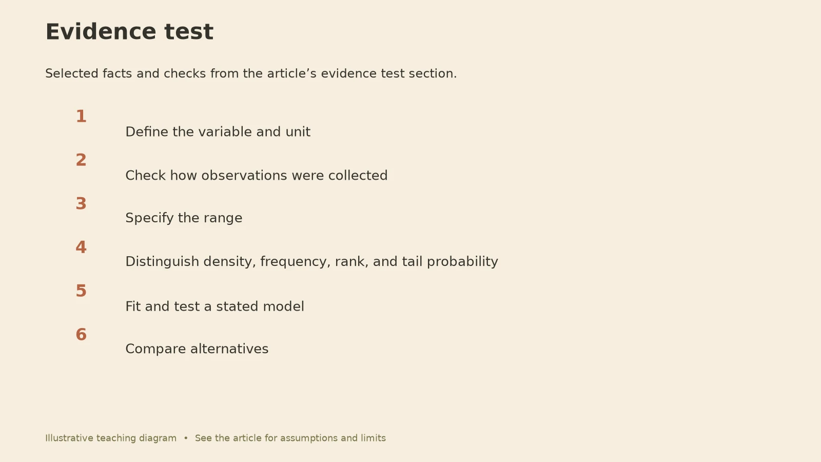
1. Find where the tail starts. Power laws usually apply only above some minimum value, and that cut-off has to be estimated from the data rather than chosen by eye.
2. Fit the exponent by maximum likelihood. Fitting a straight line to a log-log histogram — the method most people reach for — produces substantially biased exponents, which was one of the central complaints in the 2009 paper.
3. Test the fit. Compare the fitted model against synthetic samples drawn from it. Clauset and colleagues suggest rejecting the power-law hypothesis when the resulting p-value falls below 0.1.
4. Compare it with the alternatives. Run a likelihood-ratio test against a lognormal and an exponential. If a rival wins, you do not have a power law — you have a heavy-ish tail, which calls for different maths.

Free implementations exist for both common languages: the powerlaw package in Python (Alstott and colleagues) and poweRlaw in R (Gillespie).

What people usually do	What it actually shows	What to do instead
Plot on log-log and look for a line	Almost any heavy tail looks straight over a short range	Fit and test the tail, not the whole dataset
Fit a regression line to that plot	A biased exponent	Maximum-likelihood estimation
Stop once the power law “fits”	Nothing — you can always fit one	Compare against the lognormal and exponential
Report R² as evidence	Very little; R² is high for the wrong model too	Report the goodness-of-fit p-value and the likelihood ratio

The Power Law in Business and Investing: Peter Thiel’s Insight

Peter Thiel, co-founder of PayPal and Palantir, popularized the power law in the startup world. In his book ‘Zero to One,’ he argues that venture capital returns follow a power law: a single successful investment can return more than all other investments combined.

This means that investors should not diversify broadly, but instead focus on the few companies that have the potential to become huge. As Thiel puts it, ‘We don’t live in a normal world; we live under a power law.’

This insight applies beyond investing. In any endeavour, a few efforts produce most of the results — so it pays to find the handful of bets that could be enormous, and to still be standing when one of them lands.

The real numbers are harsher than 80/20 — and they change the advice

Thiel’s argument is usually compressed into “don’t diversify.” The data underneath it says something more precise.

Source	What was measured	Result
Horsley Bridge	~7,000 venture investments, 1975–2014	~6% of investments, about 4.5% of dollars deployed, produced ~60% of total returns
Correlation Ventures	Thousands of US venture financings	~65% of deals returned less than the capital invested; ~4% returned over 10×; ~0.4% returned over 50×
AngelList	Tens of thousands of early-stage deals	The median investment lost money while the top 1% generated most of the gains

The Horsley Bridge figures were published by Andreessen Horowitz in 2015 and later used by Sebastian Mallaby in The Power Law; the Correlation Ventures numbers come from its analysis of Dow Jones VentureSource data.

Set against the familiar 80/20 rule, this is closer to 60/6 — considerably more extreme than most people picture. But look at what follows from it. If 6% of investments carry the result, and nobody can reliably identify that 6% in advance, the rational response is not a smaller portfolio. It is enough attempts to have a realistic chance of touching an outlier, plus the capital and the access to keep backing it once it starts working. Andreessen Horowitz called this the Babe Ruth effect: the strike-out rate is the wrong thing to minimise.

So concentration only beats breadth if you can pick the winner beforehand — and the very datasets that establish the power law also show that investors cannot. That is the difference between a description and a strategy. A power law tells you the shape of the outcomes. It never tells you which item will be the big one, and it never says “bet everything on one”.

How the Power Law Is Actually Used in Practice

A distribution is only useful if it changes a decision. Here is what people in different fields actually do once they accept that they are working with a heavy tail.

Insurance: price the layers, not the average

An insurer facing storm or flood risk cannot work from an average claim, because a single event produces thousands of correlated claims at once. So the risk gets sliced vertically instead. The insurer keeps losses up to a threshold, buys an excess-of-loss layer above that threshold, and buys further layers above that one.

Each layer is priced separately because each is driven by a different part of the same distribution: lower layers are dominated by frequent, moderate events, while higher layers are dominated by rare, severe ones (Risks 9(3):52, 2021). In this industry the fat tail is not an inconvenience — it is the product being sold.

Cities: the exponent tells you what scales and what doesn’t

Bettencourt, West and colleagues (PNAS, 2007) measured how city metrics change with population. Socioeconomic output — wages, patents, economic activity — grows superlinearly, with an exponent around 1.15, so doubling a city’s population raises output by more than double. Infrastructure such as road surface, cable length and petrol stations grows sublinearly, with an exponent around 0.85, so double the people need only about 85% more infrastructure.

Planners use those two exponents directly: they set the expectation for per-capita infrastructure cost as a city grows, and they provide a baseline to judge whether a particular city is over- or under-performing for its size. The same method shows that some undesirable quantities also scale superlinearly, which is why big cities are more productive and more congested at once.

Publishing: plan for the median, finance the tail

When 98% of new titles sell under 5,000 copies, an editor cannot run the business on the average book. Publishing houses respond the way a venture fund does: a broad list where most titles roughly cover themselves, a small number of expected hits that fund everything else, and a backlist of proven sellers that provides the stable base. The mistake the numbers guard against is treating a bestseller as the normal case that failed to happen.

Operations: the Pareto chart

The Pareto chart — defect causes as descending bars, with a cumulative percentage line across the top — is one of the seven basic tools of quality control, and it exists to answer one question: which few causes account for most of the failures? It is the plainest everyday use of the idea. One caveat worth keeping: the two numbers do not have to add to 100. Sometimes 20% of causes drive 50% of the problem, sometimes 99%. Measure your own split rather than assuming 80/20.

Policy: the exponent as a dial

Economists summarise the top of the wealth distribution with a Pareto exponent, where a lower exponent means a fatter top tail. Gomez and Gouin-Bonenfant estimate that a permanent one-percentage-point fall in the required return on wealth lowers that exponent by around 42 log points, which accounts for between a third and a half of the fattening of the US wealth distribution between 1985 and 2015. That turns “inequality rose” into a quantity that can be attributed to specific causes.

Field	What they measure	What the power law changes
Insurance	Loss size above thresholds	Risk is sold in separately priced layers instead of averaged
Urban planning	Output and infrastructure vs population	Per-capita cost forecasts and city benchmarking
Publishing	Copies per title	Broad lists, backlist reliance, advances sized for the median
Venture and product	Return per bet	More attempts plus follow-on capital, not fewer bets
Quality and operations	Defects per cause	Fix the few causes that dominate failures
Public policy	Top-tail wealth share	Inequality changes get attributed to measurable drivers

Why the Average Betrays You, and How Much Data It Would Take to Fix It

Everyone repeats that averages are misleading in a power-law world. Almost nobody says by how much, and the size of the gap is genuinely startling.

In a bell-curve world, roughly 30 observations are enough to pin the mean down to a given precision. Under a Pareto 80/20 tail, reaching that same precision can take on the order of 10¹¹ observations — a hundred billion (Taleb, Statistical Consequences of Fat Tails, arXiv:2001.10488, and his Darwin College lecture “Probability, Risk, and Extremes”). Nobody has a hundred billion observations of startup exits, wildfire losses or book sales. The practical consequence is that in these datasets your sample mean is not a slightly noisy estimate of the truth; it is a number that will keep moving whenever a new large observation arrives.

How bad it gets depends on the exponent:

Exponent	What still works
Above 3	Ordinary statistics behave more or less as taught
Between 2 and 3	Mean and variance exist, but estimates converge painfully slowly
Between 1 and 2	The mean exists; the variance is infinite, so standard deviation and correlation stop being meaningful
1 or below	Even the mean does not exist

Remember the Forbes 400 exponent of about 1.49. It sits in the infinite-variance band, which means “average billionaire wealth plus or minus a standard deviation” is not a statement that carries information.

What to do instead, in order of usefulness:

1. Report the median alongside the mean, and say plainly which one answers the reader’s question.
2. Report a top share — the share of the total held by the largest 1% or 10% of observations. This is the number that actually describes concentration.
3. Check what fraction of your total comes from your single largest observation. If one item is 30% of the total, you are in tail territory and no summary statistic will rescue you.
4. Prefer mean absolute deviation to standard deviation, since squaring gives outliers enormous extra weight.
5. Never lead with correlation or R² on this kind of data.

Common Mistakes When Thinking About Power Laws

1. Assuming everything is a power law: Plenty of skewed data is lognormal, exponential or simply messy. Since a power law can always be fitted, fitting one proves nothing on its own — run the comparison test.
2. Ignoring the threshold: A power law usually holds only above a minimum value. Estimate that cut-off; if you fit the whole dataset including the small values, you will get an exponent that describes neither end of it.
3. Confusing a time trend with a distribution: “Quantity grows as a power of time” and “the sizes of things follow a power law” are two different claims with different evidence. Bitcoin models mix them up constantly.
4. Confusing correlation with causation: A power-law fit describes a shape. It says nothing about what produced it, and several very different mechanisms produce the same shape.
5. Using the average: In a power-law world the mean drifts with every new outlier. Use the median plus a top-share figure.
6. Overestimating predictability: A power law tells you that large events are more likely than a bell curve implies. It does not tell you when the next one arrives, or which candidate will be the outlier.

Practical Takeaways: How to Use the Power Law in Your Life

• Measure your own split before trusting 80/20: Rank your customers, projects or bug reports by contribution and read off the real numbers. Venture returns run near 60/6; your case might be 50/20. The ratio you assume determines how aggressively you should cut.
• Buy more attempts, cap each downside: In power-law fields the useful lever is the number of shots you can survive, not the confidence behind any single one. Keep each bet small enough that a total loss is not fatal, and keep enough capital in reserve to double down on whatever starts working.
• Set expectations from the median, not the headline: Most books sell a few hundred copies and most startups do not return their capital. Planning against the median keeps you solvent long enough for a tail outcome to be possible.
• Test the assumption before you act on it: Ask whether a power law or a lognormal fits better. The two look alike on a chart and imply very different worst cases, and that difference is what your risk budget rests on.

Frequently Asked Questions

What is power law in simple terms?

A power law is a relationship where a change in one quantity leads to a proportional change in another, regardless of size. It creates a pattern where a few large events dominate, and many small ones are common. For example, a few cities have most of the population, and a few people have most of the wealth.

What is power law by Peter Thiel?

Peter Thiel, in his book ‘Zero to One,’ describes how venture capital returns follow a power law: a single successful startup can return more than all others combined. He advises investors to focus on the few companies with the potential for massive growth rather than diversifying broadly.

What is meant by the power law?

The power law is a mathematical relationship where one quantity varies as a power of another. It often appears in natural and social systems, producing distributions with ‘fat tails’ where extreme events are more common than expected under a normal distribution.

What is the 3 formula of power?

In physics, the formula for power is P = W/t (power equals work divided by time). In the context of power laws, the general formula is y = a × x^k, where k is the exponent. There isn’t a “3 formula” specifically; the phrase probably refers to the three forms of the power equation in electricity: P = VI, P = I²R, and P = V²/R.

Can you give me an example of a power law?

A classic example is the distribution of city populations. If you rank cities by population, the largest is about twice the second, three times the third, and so on. This is known as Zipf’s law, a type of power law.

Does Bitcoin follow the power law?

Bitcoin’s price plotted against its age does form a strikingly straight line on a log-log chart — a model popularised by physicist Giovanni Santostasi, with a fitted exponent close to 6. Treat it as a curve fit rather than a law.

A 2026 analysis posted on arXiv, Bitcoin’s Power Law: Weak Structure, Strong Forecasts, reported two problems. The distributional power law is rejected for UTXO balances and for daily absolute returns, with the lognormal decisively preferred. And the fitted time-domain exponent varies by nearly a factor of three depending on where the time origin is placed, which is not the behaviour a genuine structural power law should show. The forecasts can still look good while the underlying structure is not what the model claims — and as noted above, “price grows as a power of time” is a different claim from “the distribution is a power law”.

Is the 80/20 rule the same thing as a power law?

Not quite. The Pareto principle is one point read off a power-law curve, popularised after Vilfredo Pareto observed that about 80% of Italian land was owned by 20% of the population. Two things are worth remembering. The numbers do not have to add up to 100 — 20% of causes might produce 50% of results, or 99%. And the split depends entirely on the exponent, which is why venture returns come out closer to 60/6 than 80/20. Measure your own ratio instead of assuming it.

How do I check whether my own data follows a power law?

Four steps, in order: estimate where the tail begins, fit the exponent by maximum likelihood rather than by drawing a line through a log-log plot, test the fit against synthetic samples from the fitted model, then run a likelihood-ratio test against a lognormal and an exponential. If a rival distribution wins, you have a heavy tail but not a power law. The powerlaw package for Python and poweRlaw for R implement all four steps, so this is an afternoon of work rather than a research project.

Conclusion: Embrace the Extremes

Power laws are a fundamental pattern in the universe, from the distribution of galaxies to the spread of viral content. By understanding this concept, you can make better decisions, set realistic expectations, and recognize when you’re in a ‘winner-take-all’ environment.

The next time you see a chart with a few towering bars and a long tail, remember: that’s not an anomaly. That’s a power law at work.

So, whether you’re an investor, a creator, or just a curious mind, keep an eye out for power laws. They might just change how you see the world.