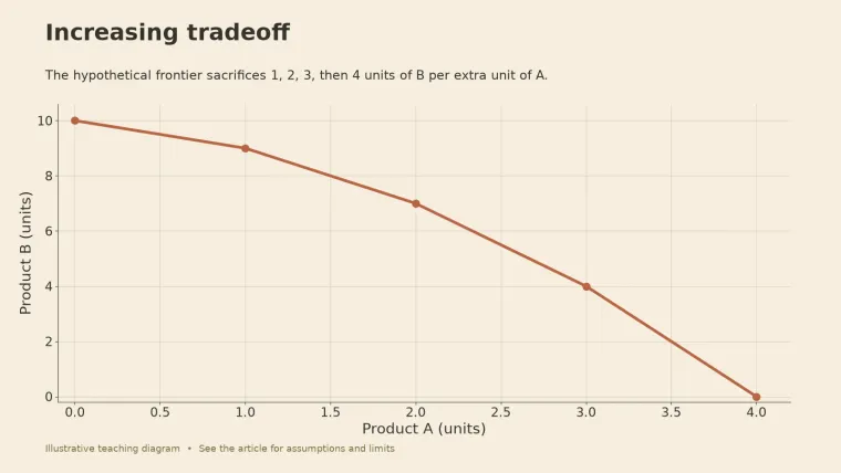
In 1940, 14.6 percent of the American labor force was unemployed. By 1944 the rate was 1.2 percent, a record low. In between, war-related production rose from about 2 percent of national output to 40 percent, according to EH.net’s history of the wartime economy. The first planes and tanks cost the country little in civilian goods. The later ones cost far more.
The law of increasing opportunity cost says that as you shift resources toward producing more of one good, each extra unit tends to require giving up more of another. It happens because resources differ in how well they suit each use. On a production possibilities frontier, the curve gets steeper.
America’s war economy shows why the later units cost more
Stage 1: idle resources. In 1940 millions of workers were still unemployed. Putting them to work on armaments did not require taking much away from civilians. Because total output grew so fast, EH.net notes, spending in many civilian sectors rose even as the war absorbed billions of dollars. The economy was starting from a point inside its frontier, so this early phase sits outside the law itself.
Stage 2: converting resources built for something else. Once slack ran out, more war output had to come from factories and workers suited to civilian goods. Car plants were the obvious target; union leader Walter Reuther had proposed turning them over to aircraft in 1940. Automakers, worried about market share, resisted. They fully converted only in 1942 and began contributing substantially to aircraft production only in 1943. A plant built for cars, asked to build planes, is the textbook poorly suited resource. Meanwhile the military curtailed civilian production of goods such as automobiles.
Stage 3: hitting the edge. In late 1942, planners fought what became known as the “feasibility dispute.” War Production Board chief Donald Nelson argued that “all-out” production for 1943 would damage the country’s ability to keep producing later, and he persuaded the military to scale back its demands. The government also began rationing steel, aluminum, and copper among users through the Controlled Materials Plan.
The record gives no neat number for the sacrifice per extra plane, but it shows the shape the law predicts: cheap gains from idle and well-suited resources first, then rising sacrifice as poorly suited resources are pulled in.
Inside the frontier versus along it
A production possibilities frontier, or PPF, describes feasible efficient combinations under specified resources and technology. Movement along a frontier changes the combination of goods while holding the production conditions fixed. A point inside the frontier leaves capacity unused, which is where the United States started in 1940. A point outside is infeasible under the stated conditions.
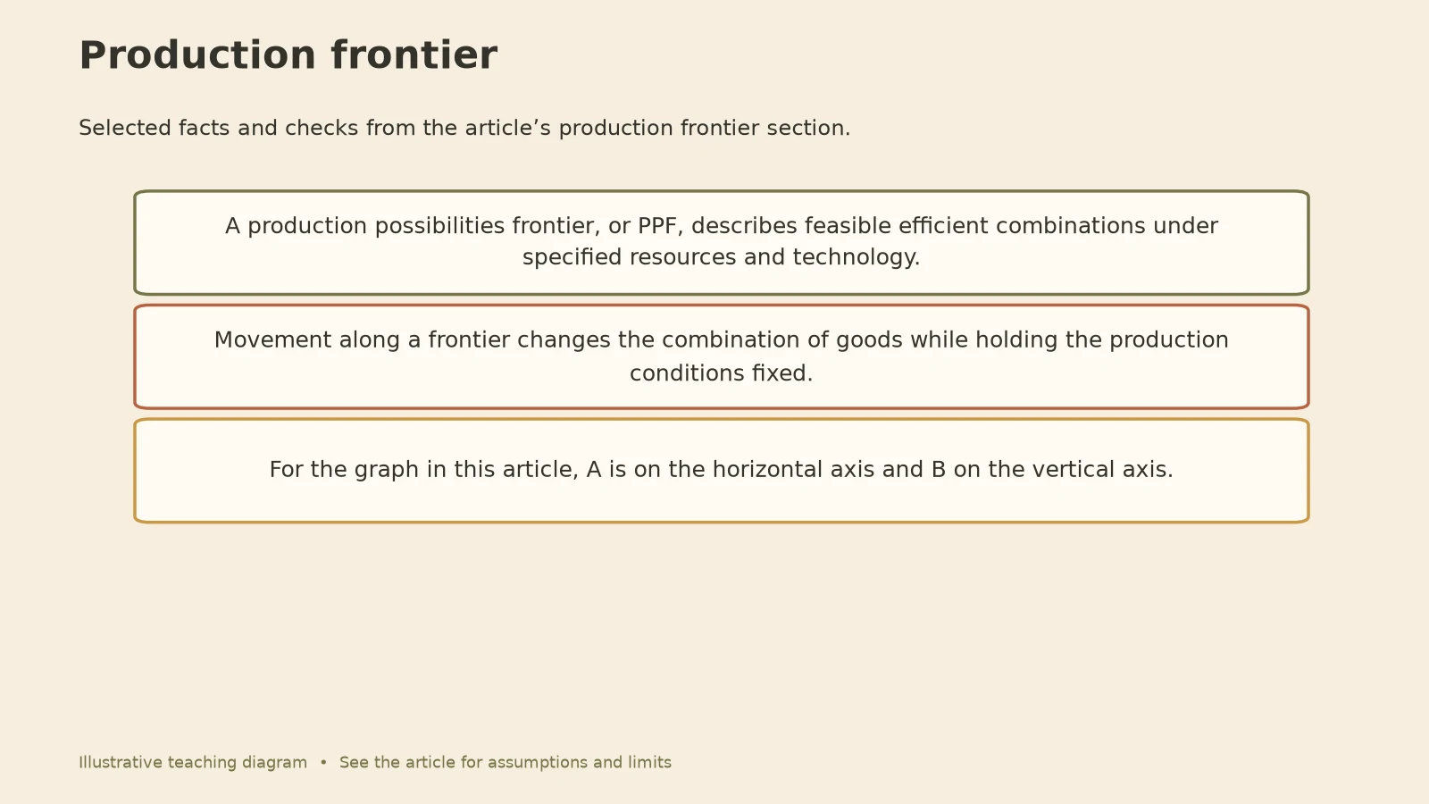
For the graph in this article, A is on the horizontal axis and B on the vertical axis. OpenStax’s production-frontier chapter links the bowed-out shape to resource specialization. A shift of the whole frontier is different again: it happens when resources or technology change, as when converted plants finally learned to build aircraft at scale.
A simple table makes the rise visible
Here is a hypothetical version, in units per production period.
| Product A | Product B | Extra A from previous row | B forgone | Opportunity cost per extra A |
|---|---|---|---|---|
| 0 | 10 | — | — | — |
| 1 | 9 | 1 | 1 | 1 B per A |
| 2 | 7 | 1 | 2 | 2 B per A |
| 3 | 4 | 1 | 3 | 3 B per A |
| 4 | 0 | 1 | 4 | 4 B per A |
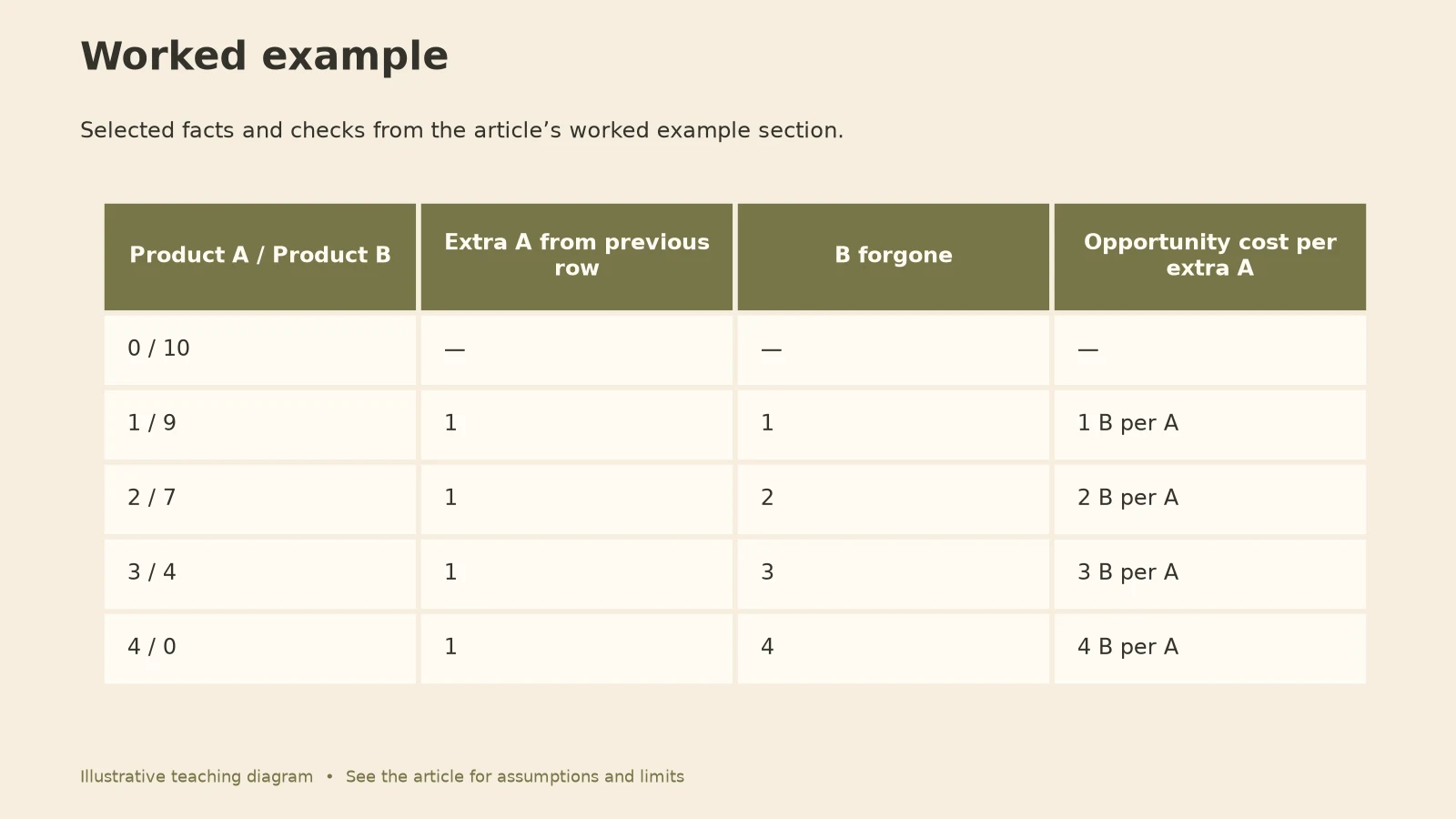
The first extra A costs one B, the next costs two, then three, then four. The marginal opportunity cost rises. If the steps in A were unequal, you would divide B forgone by the extra A in each interval. The opportunity cost formula guide walks through that calculation.
Constant, increasing, or decreasing
| Pattern | Illustrative B sacrifices for equal A increments | Frontier implication in the simple model |
|---|---|---|
| Increasing opportunity cost | 1, 2, 3, 4 | The tradeoff becomes steeper |
| Constant opportunity cost | 2, 2, 2, 2 | A straight-line tradeoff |
| Decreasing opportunity cost | 4, 3, 2, 1 | The tradeoff becomes less steep |
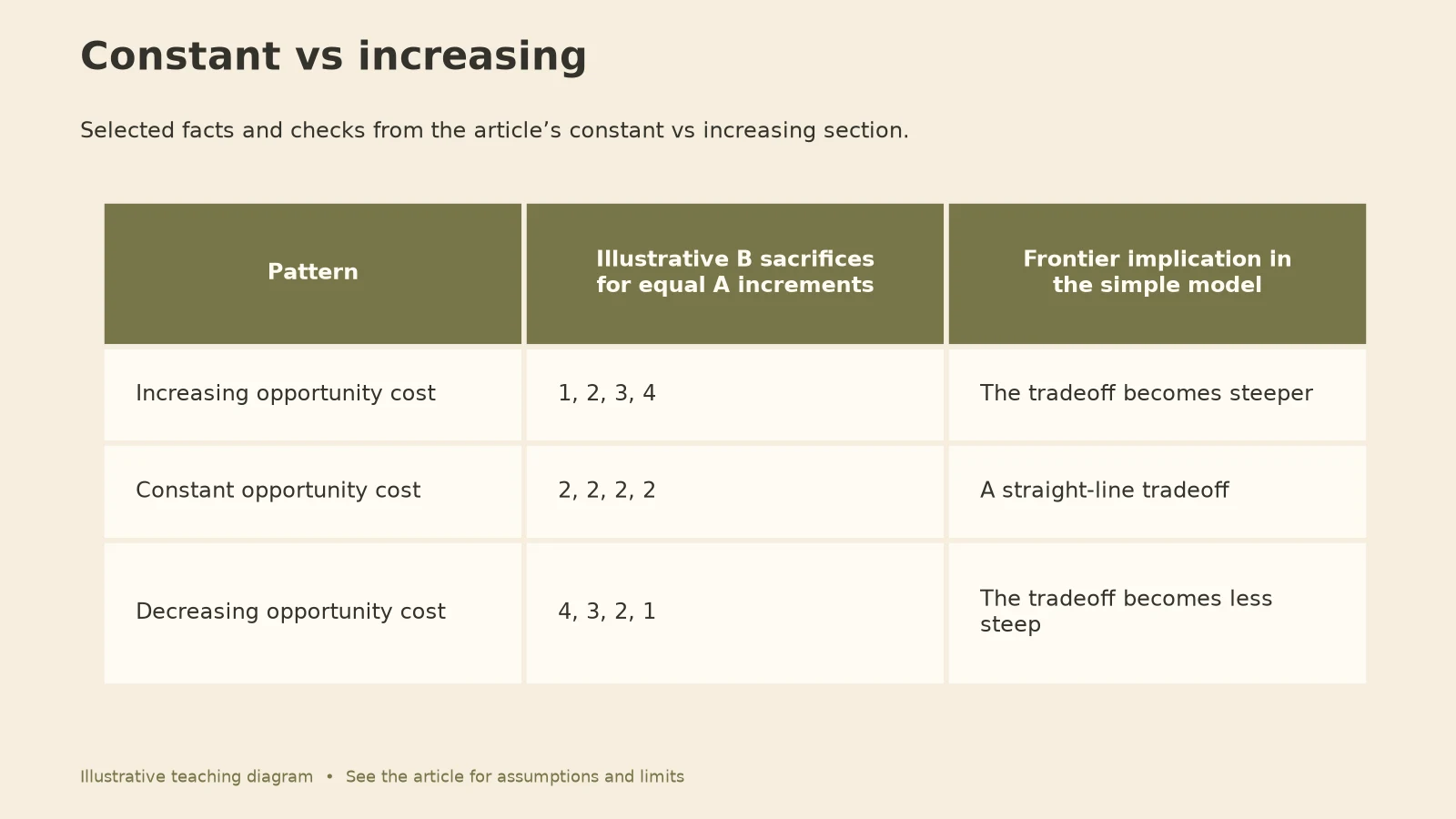
Which pattern a real process follows depends on its resources, technology, scale, and the range examined. Interchangeable resources give something close to a constant tradeoff. Highly specialized resources, like a 1941 car plant asked to build bombers, produce the steep part of the curve.
When the law misleads
Assuming it without evidence. The law describes a common condition, not a guarantee that every frontier bows outward.
Mistaking slack for a free lunch. Early wartime gains came from idle resources. Once the slack is gone, the same move costs much more. Check where you start before extrapolating.
Confusing opportunity cost with price. A firm’s bill can rise for reasons unrelated to resource suitability. This law concerns goods forgone, not market prices.
Forgetting that time moves the frontier. Retraining and retooling can turn poorly suited resources into well-suited ones. A cost that looks steep this quarter may flatten after conversion.
For the core idea, see opportunity cost. For how a compromise differs from the value of the best alternative, see trade-off vs opportunity cost.
Questions
Why does opportunity cost increase?
In the standard explanation, resources differ in suitability. As production moves further toward one good, resources better suited to the other good must be reassigned, so each extra unit sacrifices more.
Is the law the same as diminishing returns?
They are related but answer different questions. Increasing opportunity cost compares goods forgone along a frontier. Diminishing returns concerns the extra output from adding more of one input while others stay fixed.
Can opportunity cost stay constant?
Yes, over a range where resources are interchangeable. Check the quantities instead of assuming every frontier has the same shape.
What is a real-world example?
US mobilization in World War II: idle workers made early war output cheap, while converting car plants to aircraft came later and slowly.
Your 5-minute frontier check
Two outputs competing for the same resources:
Am I starting with slack (idle people, spare capacity)? yes / no
Which resources are best suited to the output I want more of?
Which would I have to pull in next, and how poorly do they fit?
Cost of the last unit vs the next unit (in units of the other output):
What retraining or retooling could flatten the curve?
For practice on real cases, take one story from Daily Read about a company scaling up or a government shifting spending, and ask where the steep part of its curve begins. To plan the choice itself, use decision-making frameworks.